
Box Cox Transformation with SigmaXL
Box Cox Transformation
- Data transforms are usually applied so that the data appear to more closely meet assumptions of a statistical inference model to be applied or to improve the interpret-ability or appearance of graphs.
- Power transformation is a class of transformation functions that raise the response to some power. For example, a square root transformation converts X to X1/2
- Box Cox transformation is a popular power transformation method developed by George E. P. Box and David Cox.
Box Cox Transformation Formula
The formula of the Box Cox transformation is:
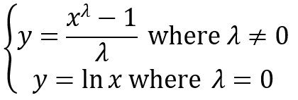
Where:
- y is the transformation result
- x is the variable under transformation
- λ is the transformation parameter
Use SigmaXL to Perform a Box-Cox Transformation
SigmaXL provides the best Box-Cox transformation with an optimal λ that minimizes the model SSE (sum of squared error). Here is an example of how we transform the non-normally distributed response to normal data using Box-Cox method.
Data File: “Box-Cox” tab in “Sample Data.xlsx”
Step 1: Test the normality of the original data set.
- Select the entire range of “Y” in column H
- Click SigmaXL -> Graphical Tool -> Histograms & Descriptive Statistics
- A new window named “Histograms & Descriptive” pops up and the selected range automatically appears in the box below “Please select your data”.
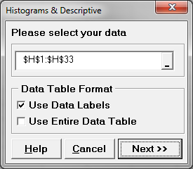
- Click “Next >>”
- A new window named “Histograms & Descriptive Statistics” pops up.
- Select “Y” as “Numeric Data Variables (Y)”
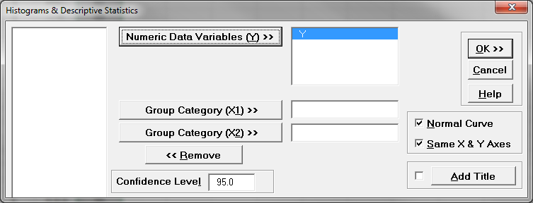
- Click “OK>>”
- The analysis results are shown automatically in the new spreadsheet “Hist Descript(1)”
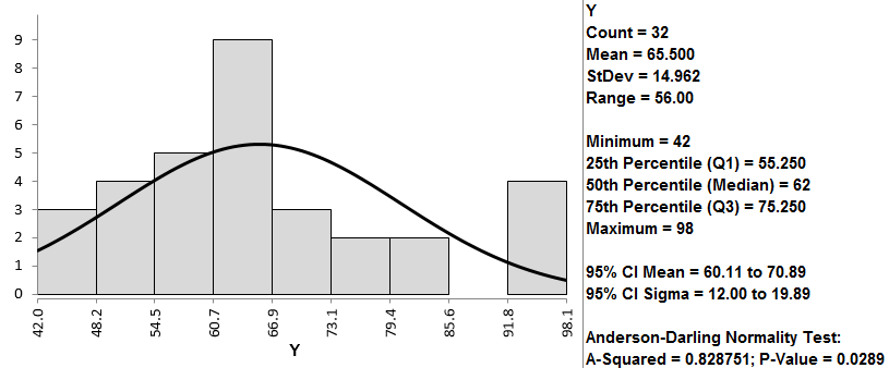
Normality Test:
- H0: The data are normally distributed.
- H1: The data are not normally distributed.
If p-value > alpha level (0.05), we fail to reject the null hypothesis. Otherwise, we reject the null. In this example, p-value = 0.029 < alpha level (0.05). The data are not normally distributed.
Step 2: Run the Box-Cox Transformation:
- Select the entire range of Y in column H
- Click SigmaXL -> Process Capability -> Nonnormal -> Box-Cox Transformation
- A new window named “Box-Cox Transformation” pops up and the selected range appears automatically in the box under “Please select your data”

- Click “Next >>”
- A new window also named “Box-Cox Transformation” pops up.
- Select “Y” as “Numeric Data Variables (Y)”
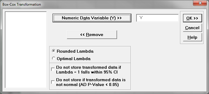
- Click “OK>>”
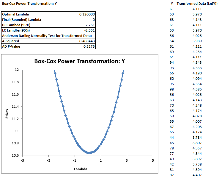
- The analysis results are shown automatically in the new spreadsheet “Box-Cox (1)”
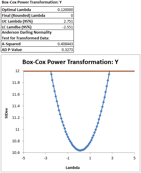
The software looks for the optimal value of lambda that minimizes the SSE (Sum of Squares of Error). In this case the minimum value is 0.12. The transformed Y can also be saved in another column. The transformed Y is also listed in Column G in the newly generated tab “Box-Cox (1)
 Use the Anderson–Darling test to test the normality of the transformed data
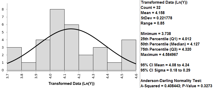
- H0: The data are normally distributed.
- H1: The data are not normally distributed.
Model summary: If p-value > alpha level (0.05), we fail to reject the null. Otherwise, we reject the null. In this example, p-value = 0.327 > alpha level (0.05). The data are normally distributed.